Lenstra–Lenstra–Lovász lattice basis reduction algorithm
The LLL-reduction algorithm (Lenstra–Lenstra–Lovász lattice basis reduction) is a polynomial time lattice reduction algorithm invented by Arjen Lenstra, Hendrik Lenstra and László Lovász in 1982, see Lenstra, Lenstra & Lovász 1982. Given as input a basis  with n-dimensional integer coordinates, for a lattice L in Rn with
  , the LLL algorithm outputs an LLL-reduced (short, nearly orthogonal) lattice basis in time
 .
.
where B is the largest of the lengths of the  under the Euclidean norm.
The original applications were to give polynomial time algorithms for factorizing polynomials with rational coefficients into irreducible polynomials, for finding simultaneous rational approximations to real numbers, and for solving the integer linear programming problem in fixed dimensions.
Contents |
LLL reduction
The precise definition of LLL-reduced is as follows: Given a basis
with its Gram–Schmidt process orthogonal basis,

define
 , for any
  .
.
Then the basis  is LLL-reduced if there exists a parameter
  in (0.25,1] such that the following holds:
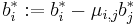
- (size-reduced) For
 . By definition, this property guarantees the length reduction of the ordered basis.
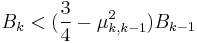
 - (Lovász condition) For k = 2,3,..,n
 .
.
Here, estimating the value of the parameter, we can conclude how well the basis is reduced. Greater values of lead to stronger reductions of the basis. Initially, A. Lenstra, H. Lenstra and L. Lovász demonstrated the LLL-reduction algorithm for  . Note that although LLL-reduction is well-defined for
  , the polynomial-time complexity is guaranteed only for in (0.25,1).
The LLL algorithm computes LLL-reduced bases. There is no known efficient algorithm to compute a basis in which the basis vectors are as short as possible for lattices of dimensions greater than 4. However, an LLL-reduced basis is nearly as short as possible, in the sense that there are absolute bounds  such that the first basis vector is no more than
  times as long as a shortest vector in the lattice, the second basis vector is likewise within
  of the second successive minimum, and so on.
LLL Algorithm
The following description is based on (Cohen 2000, Algorithm 2.6.3), but currently is incorrect.
INPUT:
 a lattice basis
  ,
,- parameter with

PROCEDURE:
Perform Gram-Schmidt:

- for
 from
from  to
to  do
do

- for
 from
from  to
to  do
do
- end for

- end for
 (k is the stage at which the vectors
  are reduced according to size-reduced property 1.)
- if
 then execute reduction subroutine RED(k,k-1):
- for
 from
from  to do
to do


- for from to
 do
do
- end for

- end for
- for
- end if
- Calculate
 for 1
for 1  and
and  for from 1 to


- while
 do
do
- Length reduce
 and correct
  according to reduction subroutine in step 4, for from 1 till
 - if
 then
then
- Exchange and

 := max
- Exchange
- else
- end if
- Length reduce
- end while

OUTPUT: LLL reduced basis 
Example
The following presents an example due to W. Bosma.[1]
INPUT:
Let a lattice basis  , be given by the columns of
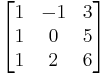
Then according to the LLL algorithm we obtain the following:
1.
2.For  DO:
DO:
2.1.For  set
set 
and 
2.2
3. 
4.Here the step 4 of the LLL algorithm is skipped as size-reduced property holds for 
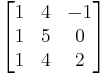
5.For  and for
  calculate and :
hence 
and 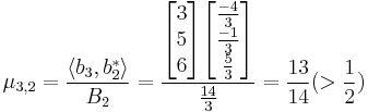
hence 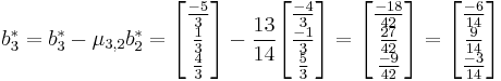 and
and

6.While  DO
DO
6.1 Length reduce  and correct
  and
and  according to reduction subroutine in step 4:
For  EXECUTE reduction subroutine RED(3,1):
i. and
and 
ii.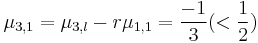
iii.Set 
For  EXECUTE reduction subroutine RED(3,2):
i.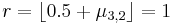 and
and 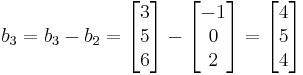
ii.Set 
iii.
6.2 As  takes place, then
6.2.1 Exchange and 
6.2.2 := 2
Apply a SWAP, continue algorithm with the lattice basis, which is given by columns
Implement the algorithm steps again. 1.
2. 
3. .
.
4. .
.
5.For  EXECUTE reduction subroutine RED(2,1):
i. and
and 
ii.Set 
6. As  takes place, then
7. Exchange and 
OUTPUT: LLL reduced basis

Applications
The LLL algorithm has found numerous other applications in MIMO detection algorithms and cryptanalysis of public-key encryption schemes: knapsack cryptosystems, RSA with particular settings, NTRUEncrypt, and so forth. The algorithm can be used to find integer solutions to many problems.[2]
In particular, the LLL algorithm forms a core of one of the integer relation algorithms. For example, if it is believed that r=1.618034 is a (slightly rounded) root to a quadratic equation with integer coefficients, one may apply the LLL reduction to the lattice in  spanned by
 ![[1,0,0,10000r^2], [0,1,0,10000r],](/2012-wikipedia_en_all_nopic_01_2012/I/3a09d44bae250cffef3372ccbf8ecfe0.png) and
and ![[0,0,1,10000]](/2012-wikipedia_en_all_nopic_01_2012/I/2594c427d5b4fb0cede2634481fcdd22.png) . The first vector in the reduced basis will be an integer linear combination of these three, thus necessarily of the form
. The first vector in the reduced basis will be an integer linear combination of these three, thus necessarily of the form ![[a,b,c,10000(ar^2%2Bbr%2Bc)]](/2012-wikipedia_en_all_nopic_01_2012/I/c96def9c2898d637a08c9361591cff70.png) ; but such a vector is "short" only if a, b, c are small and
; but such a vector is "short" only if a, b, c are small and  is even smaller. Thus the first three entries of this short vector are likely to be the coefficients of the integral quadratic polynomial which has r as a root. In this example the LLL algorithm finds the shortest vector to be [1, -1, -1, 0.00025] and indeed
  has a root equal to 1.6180339887…(The Golden Ratio)
Implementations
LLL is implemented in
- Arageli as the function lll_reduction_int
- fpLLL as a stand-alone implementation
- GAP as the function LLLReducedBasis
- LiDIA as the function/method lll in the LT package
- Macaulay2 as the function LLL in the package LLLBases
- Magma as the functions LLL and LLLGram (taking a gram matrix)
- Maple as the function IntegerRelations[LLL]
- Mathematica as the function LatticeReduce
- Number Theory Library (NTL) as the function LLL
- PARI/GP as the function qflll
- Sage as the method LLL driven by fpLLL and NTL
See also
Notes
- ^ Bosma, Wieb. "4. LLL". Lecture notes. http://www.math.ru.nl/~bosma/onderwijs/voorjaar07/compalg7.pdf. Retrieved 28 February 2010.
- ^ D. Simon (2007). "Selected applications of LLL in number theory". LLL+25 Conference (Caen, France). http://www.math.unicaen.fr/~simon/maths/lll25_Simon.pdf.
References
- Borwein, Peter (2002). Computational Excursions in Analysis and Number Theory. ISBN 0-387-95444-9.
- Cohen, Henri (2000). A course in computational algebraic number theory. GTM. 138. Springer. ISBN 3540556400.
- Lenstra, A. K.; Lenstra, H. W., Jr.; Lovász, L. (1982). "Factoring polynomials with rational coefficients". Mathematische Annalen 261 (4): 515–534. doi:10.1007/BF01457454. MR0682664. hdl:1887/3810.